The positioning of smartphones is essential for many applications. Unfortunately, the accuracy of the individual smartphone sensors often does not meet the requirements regarding accuracy. In this article the problem is discussed and solved by combining insividaul sensor values. The aproach is based on the Kalman filter. This filter combines several sensors values into one sensor of higher accuracy than the individual sensor accuracy. The Kalman filter can be realized by different methods. In this article the Kalman filter is based on the method called sensor fusion. The filter converts all sensor data into quaternions for the state estimation and correction procedure and further for the precise position determination. The evaluation proves that the combined sensor data achieves better position determination than the individual sensors.

Introduction

The position determination of a smartphone is of major importance for many applications. Whether for controlling games, for evaluating one’s own physical activity or for recognizing a person who has fallen, the situation should always be determined as accurately as possible. Smartphones have various sensors, such as acceleration, gyro and compass sensors. Unfortunately, the accuracy of single sensors often does not meet the requirements for accurate position determination.

In this project the acceleration and the gyro sensor are used to determine the position of the smartphone. The Kalman filter is used to take advantage of the positive properties of both sensors. The Kalman filter has the ability to make better estimations about the real system state for given measurement values from different sources. For instance, the Kalman filter was successfully used for the navigation of NASA’s Apollo program ¹.

In the literature study, two methods for implementing the Kalman filter are examined in more detail. These are the methods sensor fusion and extended Kalman filter (EKF) ², ³. During sensor fusion the dependency of states and errors are calculated by linear matrix operations. Therefore all sensor data must be converted into quaternions. This method can only be used for linear models ³. The extended Kalman filter method describes the dependence of the states by an equation, which calculates the error by a partial derivative. The nonlinear system is represented by the Jacobi matrix. Thus the EKF can also be used for nonlinear models ³. After the literature study it was decided that only the sensor fusion will be treated in depth.

Method

The data of the acceleration and gyro sensors are first read and converted to Euler angles. In the second step the sensor data are converted into quaternions and supplied to the Kalman filter. This sensor data is fusioned with the Kalman filter and displayed graphically to the user. This process is explained in more detail in the following subsections.

Reading the Sensor Data

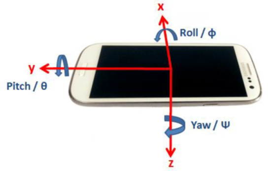
The sensor data are read and designated according to the following illustration. The axes indicate the measuring direction of the accelerometer and the angles indicate the measuring direction of the gyrometer.

With the data of the acceleration sensor the Euler angles can be calculated as follows. From the equation it can be seen that the angle \( \Psi \) cannot be determined.

$$ \begin{bmatrix} f_{x} \\ f_{y} \\ f_{z} \end{bmatrix} = g \cdot \begin{bmatrix} \sin(\Theta) \\ -\cos(\Theta) \cdot \sin(\Phi) \\ -\cos(\Theta) \cdot \cos(\Phi) \end{bmatrix} $$

$$ \Phi = \arcsin\left(\frac{-f_{y}}{g \cdot \cos(\Theta)}\right) $$

$$ \Theta = \arcsin\left(\frac{f_{x}}{g }\right) $$

The determination of the Euler angles by means of the gyrometer is realized by integration.

$$ \begin{bmatrix} \dot{\Phi} \\ \dot{\Theta} \\ \dot{\Psi} \end{bmatrix} = \begin{bmatrix} 0 & \sin{\Phi} \cdot \tan{\Theta} & \cos{\Phi} \cdot \tan{\Theta} \\ 0 & \cos{\Phi} & -\sin{\Phi} \\ 0 & \frac{\sin{\Phi}}{\cos{\Theta}} & \frac{\cos{\Phi}}{\cos{\Theta}} \end{bmatrix} \begin{bmatrix} p \\ q \\ r \end{bmatrix} $$

With these conversions the disadvantages of the acceleration and gyro sensor can be recognized. The acceleration sensor cannot determine the angle \( \Psi \) and with the gyro sensor not only the angles on are integrated, but also its error. The task of the Kalman filter is to eliminate these disadvantages of each sensor by the advantages of the other sensors.

Kalman Filter

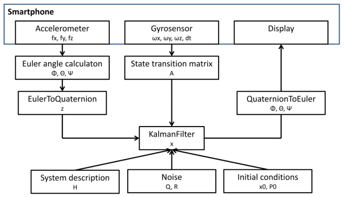
For the application of the Kalman filter the approach of sensor fusion is implemented as shown in the following figure. The sensor data must be available in quaternions as described above.

The transformation of the acceleration sensor data into Euler angles is done as described above. Subsequently, the Euler angles must be converted into quaternions. This is done with equation below ², ⁴, ⁵. The quaternions of the accelerometer are combined in the first vector.

$$ \begin{bmatrix} q_{1} \\ q_{2} \\ q_{3} \\ q_{4} \end{bmatrix} = \begin{bmatrix} \cos\left(\frac{\Phi}{2}\right) \cos\left(\frac{\Theta}{2}\right) \cos\left(\frac{\Psi}{2}\right) + \sin\left(\frac{\Phi}{2}\right) \sin\left(\frac{\Theta}{2}\right) \sin\left(\frac{\Psi}{2}\right) \\ \sin\left(\frac{\Phi}{2}\right) \cos\left(\frac{\Theta}{2}\right) \cos\left(\frac{\Psi}{2}\right) - \cos\left(\frac{\Phi}{2}\right) \sin\left(\frac{\Theta}{2}\right) \sin\left(\frac{\Psi}{2}\right) \\ \cos\left(\frac{\Phi}{2}\right) \sin\left(\frac{\Theta}{2}\right) \cos\left(\frac{\Psi}{2}\right) + \sin\left(\frac{\Phi}{2}\right) \cos\left(\frac{\Theta}{2}\right) \sin\left(\frac{\Psi}{2}\right) \\ \cos\left(\frac{\Phi}{2}\right) \cos\left(\frac{\Theta}{2}\right) \sin\left(\frac{\Psi}{2}\right) - \sin\left(\frac{\Phi}{2}\right) \sin\left(\frac{\Theta}{2}\right) \cos\left(\frac{\Psi}{2}\right) \end{bmatrix} $$

The gyro sensor uses the direct conversion of the sensor data into quaternions, which is done with the following equation ², ⁴.

$$ \begin{bmatrix} \dot{q_{1}} \\ \dot{q_{2}} \\ \dot{q_{3}} \\ \dot{q_{4}} \end{bmatrix} = \frac{1}{2} \begin{bmatrix} 0 & -p & -q & -r \\ p & 0 & r & -q \\ q & -r & 0 & p \\ r & q & -p & 0 \end{bmatrix} \begin{bmatrix} q_{1} \\ q_{2} \\ q_{3} \\ q_{4} \end{bmatrix} $$

This relationship can be discretized leading to the following system model.

$$ \begin{bmatrix} q_{1} \\ q_{2} \\ q_{3} \\ q_{4} \end{bmatrix}_{k+1} = I + dt \cdot \frac{1}{2} \begin{bmatrix} 0 & -p & -q & -r \\ p & 0 & r & -q \\ q & -r & 0 & p \\ r & q & -p & 0 \end{bmatrix} \begin{bmatrix} q_1 \\ q_2 \\ q_3 \\ q_4 \end{bmatrix}_k $$

The system matrix is summarized in \( A \). It describes the current state by the previous one.

$$ A = I + dt \cdot \frac{1}{2} \begin{bmatrix} 0 & -p & -q & -r \\ p & 0 & r & -q \\ q & -r & 0 & p \\ r & q & -p & 0 \end{bmatrix} $$

As shown in the figure above, the Kalman filter needs not only the sensor data, but also the system description, noise and start conditions. The variance matrix \( Q \) with the mean value \( 0 \) and the measurement error covariance matrix \( R \) are defined as follows ⁶.

$$ Q = 10^{-a} \begin{bmatrix} 1 & 0 & 0 & 0 \\ 0 & 1 & 0 & 0 \\ 0 & 0 & 1 & 0 \\ 0 & 0 & 0 & 1 \end{bmatrix} $$

$$ R = b \begin{bmatrix} 1 & 0 & 0 & 0 \\ 0 & 1 & 0 & 0 \\ 0 & 0 & 1 & 0 \\ 0 & 0 & 0 & 1 \end{bmatrix} $$

The variables \( a \) and \( b \) are sensor dependent and must be determined empirically. The choice of \( a = 4 \) and \( b = 10 \) provides the best results for the present system.

The Kalman filter is initialized with the values given below. This initialization assumes that the smartphone is initially positioned horizontally in the room. If this is not the case, the Kalman filter will give very deviating values at the beginning, but after a short time they converge to the effective value.

$$ x = \begin{bmatrix} 1 \\ 0 \\ 0 \\ 0 \end{bmatrix} $$

$$ P_{0}^{-} = \begin{bmatrix} 1 & 0 & 0 & 0 \\ 0 & 1 & 0 & 0 \\ 0 & 0 & 1 & 0 \\ 0 & 0 & 0 & 1 \end{bmatrix} $$

Finnaly, all parameters required by the Kalman filter are defined. The following diagram shows how the Kalman filter processes the sensor data consisting of prediction and correction.

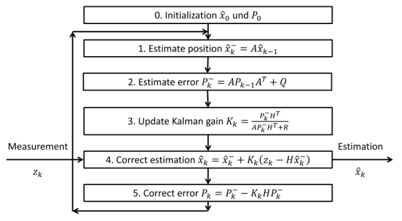
The sensor fusion method relies on the ARMA model. After initialization the Kalman filter algorithm is based on the continuous cycle of estimation and correction.

Thereby, the algorithm estimates the next value and the error of the estimate. Afterwards the sensor sources are weighted and the sensor data are read in. With the new sensor data and with the previous estimate the value is calculated and output again. The algorithm now compares the estimated error with the effective error and corrects it. The corrected error and the output value is used for the next cycle.

Displaying the Sensor Data

To get to Euler angles from the quaternions after the Kalman filter the following approach is used ², ⁷. The result of this equation can thus be displayed directly on the smartphone.

$$ \begin{bmatrix} \Phi \\ \Theta \\ \Psi \end{bmatrix} = \begin{bmatrix} \text{arctan2}\left(2 \cdot (q_{3} \cdot q_{4} + q_{1} \cdot q_{2}), 1-2(q_{2}^{2} + q_{3}^{2})\right) \\ -\arcsin\left(2 \cdot (q_{2} \cdot q_{4} - q_{1} \cdot q_{3})\right) \\ \text{arctan2}\left(2 \cdot (q_{2} \cdot q_{3} + q_{1} \cdot q_{4}), 1-2(q_{3}^{2} + q_{4}^{2})\right) \end{bmatrix} $$

Results

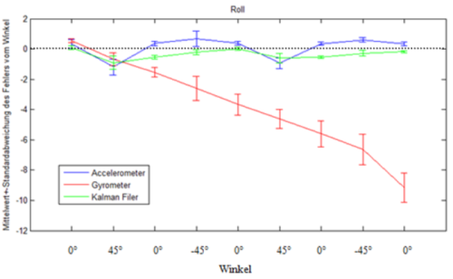
During the evaluation the angle values of the acceleration and gyro sensor are compared with the angle value of the Kalman filter. The measurement was performed using a defined dynamic procedure. The angle \( \Theta \) of the smartphone is changed every 3 seconds to the following angle values: 0°, +45°, 0°, -45°, 0°, +45°, 0°, -45°, 0. This measurement is repeated 10 times. Subsequently, the same procedure is used to record measured values for the angle \( \Phi \). The data of the accelerometer is filtered with a low pass filter of order 20 and a cut-off frequency of 10Hz ⁸.

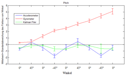
The following diagrams show the angle errors of the acceleration, gyro sensor and the Kalman filter for the angle \( \Theta \) and \( \Phi \). The errors are given as mean value and standard deviation of the 10 measurements.

Discussion

The diagrams of the evaluation show that the mean value of the acceleration sensor error remains approximately constant over time. This means that the accelerometer always has an error in the same range.

With the gyro sensor a clear increase of the error is evident. Thus the errors increase over time. This is caused due to the conversion of the gyro data into Euler angles. During the conversion not only the angles are integrated, but also the errors. Thus these increase strongly, since the gyro sensor always has a small offset error.

Both figures show that the Kalman filter combines the good characteristics of both sensors. The mean error value of the Kalman filter is always closer to zero than the mean error values of the acceleration and gyro sensor. Thus, the Kalman filter combines the two sensors to a qualitatively better sensor.

If the diagrams are compared among themselves, no larger difference can be recognized, except that the gyro sensor drifts in a different direction. This phenomena is caused by the definition of the axis. Further, it ensures that the same error phenomena occur when determining the angle \( \Theta \) as when determining the angle \( \Phi \).

For all measured values the standard deviation is approximately equal. From this it can be concluded that the angle of the test object was precisely adjusted during the measurements.

Conclusions

In this project, the feasibility of the sensor fusion method was demonstrated using the practical example of the smartphone for position determination. During the dynamic measurement an error reduction of the Euler angles could be achieved with the Kalman filter.

The method described in this paper is not adaptive regarding sensor noise. This means it does not adapt to different sensors or their properties, because the noise \( R \) and \( Q \) are defined as constants. In a further step, an automatic determination of these variables could be implemented.

The model described in this article could be extended with other sensors, such as a barometric air pressure sensor or a magnetic field sensor. This in turn would lead to a more precise determination of the position.